摘要
本文主要介绍Einstein@home项目的背景、目标和发展历史,以及拥有闲置算力的我们如何以最不费力的方式参与到大科学中,并提供相关配置教程,本文主主要参考项目官方页面,项目Wiki页面和第三方中文资料。
什么事Einstein@home
爱因斯坦@Home 是一个“2005年物理年”和“2009年国际天文学年”项目,由美国物理学会 (APS)、美国国家科学基金会 (NSF)、德国马克斯·普朗克学会 (MPG) 以及一些国际组织支持。
爱因斯坦@Home 利用您计算机的空闲时间,使用来自 LIGO 引力波探测器、MeerKAT 射电望远镜、费米伽马射线卫星以及阿雷西博射电望远镜的历史数据,寻找来自旋转中子星(通常称为脉冲星)的微弱天体物理信号。爱因斯坦@Home 的志愿者们已经发现了超过 90 颗新的中子星,我们希望能够发现更多。
我们的长期目标是实现旋转中子星引力波辐射的首次直接探测。引力波是阿尔伯特·爱因斯坦一个世纪前所预言的,并于 2015 年 9 月 14 日首次被直接探测到。这次探测来自一对合并的黑洞,开启了探索宇宙的新窗口,也标志着天文学进入了一个新时代。
这次首次直接探测是在 LIGO 设备经过为期五年的重大升级并重新上线后不久取得的。自那时以来,这些先进探测器已经完成了三次灵敏度不断提升的观测运行,发现了超过 90 次黑洞与中子星合并事件。自 2023 年 5 月起,第四次且最灵敏的观测运行已经开始,预计在 2025 年初结束前将新增约 200 次引力波探测事件。
要了解更多关于爱因斯坦@Home 的信息,请点击上方“出版物”中的链接。我们的一些项目和发现的媒体报道可在“新闻”部分查看。有关我们数据分析的更多详细信息,请参阅“数据分析”。
如果您想参与,请按照“立即加入”的说明操作。注册只需一两分钟,并且几乎不需要维护即可让爱因斯坦@Home 正常运行。爱因斯坦@Home 适用于 Windows、Linux 和 Apple macOS 计算机,以及 Android 设备。
历史成就
详情见本页内容
如何参与
一、安装BOINC客户端
该项目基于BOINC平台管理和运行,毫无疑问,第一步是安装BOINC的客户端软件,非常幸运,该软件从下载、安装到运行都是高度图形化的,这一过程在合适的网络环境下非常顺滑。以下我们将分别展示在Windows,MacOS,Linux环境下安装该软件:
- Windows
访问官方资源页面,理论上,你的系统信息将被自动识别,页面上将展示对应操作系统的软件包下载链接。若系统没能正确识别你的系统信息,请访问Download BOINC client software (berkeley.edu)选择对应你的操作系统的软件版本
- MacOS
访问官方资源页面,理论上,你的系统信息将被自动识别,页面上将展示对应操作系统的软件包下载链接。若系统没能正确识别你的系统信息,请访问Download BOINC client software (berkeley.edu)选择对应你的操作系统的软件版本
- Ubuntu/Debian
在Debian/Ubuntu下配置BOINC manager相对来说较为积遭,可以参考官方页面的步骤,实在不行就问问gpt;
另一种方法是直接使用.deb包安装,资源可以在Boinc Download (DEB, IPK, RPM, XBPS, XZ, ZST) (pkgs.org)获取
二、在BOINC客户端中添加Einstein@home项目
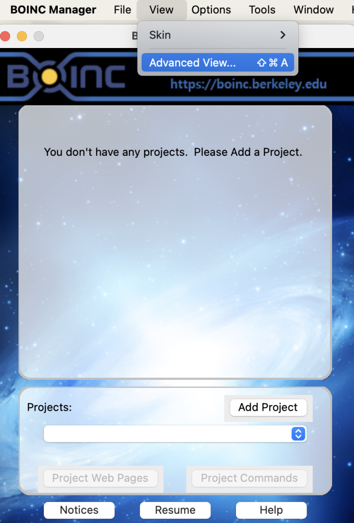
打开客户端,我忘记默认是simple view还是advanced view了,可以通过面板上的view选项更改,看你喜欢哪一种界面了。在切换到你喜欢的控制界面后,找到并点击add project按钮(如果你找不到,就换一种界面风格,据我所知人很容易找不到很明显的按钮)
这是advanced view,该界面下,点击Tools,找到add project选项
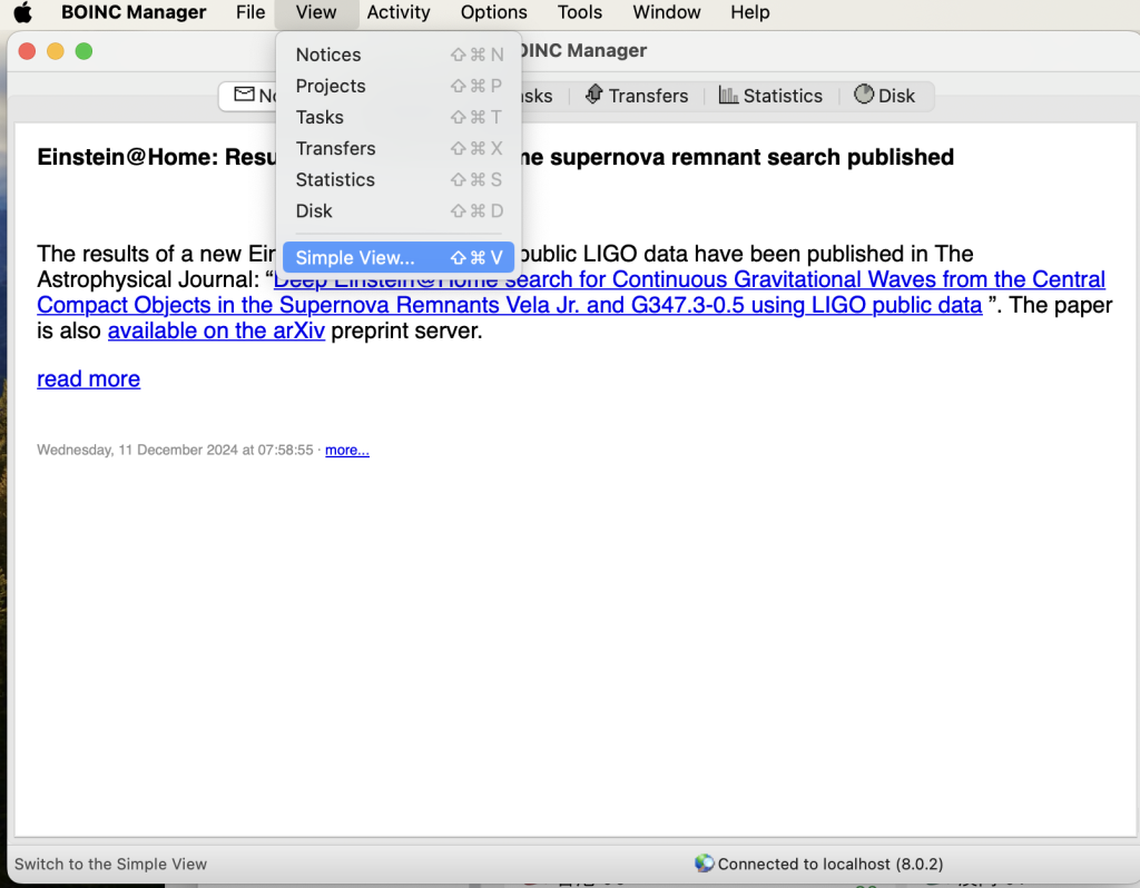
这是simple view,该界面下,直接看到Add Project按钮
注意,BOINC平台用于管理包括Einstein@home在内的数个分布式科学计算项目,在该瓶套的语境下,Projects指类似Einstein@home的科学项目,Tasks则指某项目下分配给参与者的具体计算任务。
在点击Add Project按钮后,将看到如下图所示页面:
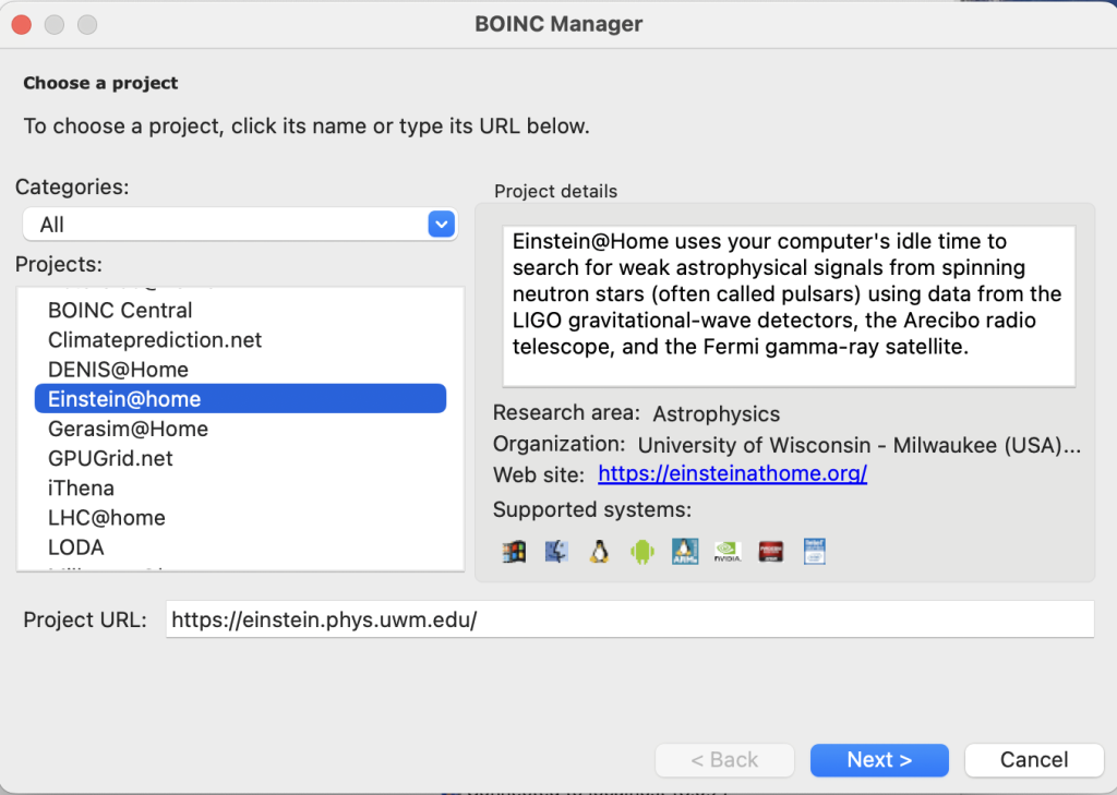
找到并选中Einstein@home或其他你感兴趣的项目,可以看到项目主页URL,可以点开看看,也可以不看直接点Next
点击Next后将与主机建立链接,时间取决于网络环境,在连接后将显示条款页面,统一并进入下一步,你将看到如图所示的注册页面,无视它!!! 你并不能通过BOINC manager注册Einstein@home账号,相反,请直接通过访问Einstein@home的注册页面注册账号,选取一个抽象的用户名并填入邮箱,注册邮件将会发至你的邮箱。

点击注册邮件中的地址,你将被重定向至设定登录密码页面,设置并找个地方记录界面中的信息,天知道什么地方有用。
现在,回到BOINC客户端,在上图页面中选取已存在的用户,使用邮箱和密码登录。不出意外的话,你会看到project added的提示,项目已经被成功添加到你的BOINC客户端
客户端和项目配置
首先介绍项目配置,在Einstein@home项目网站上,你可以管理你想要进行的任务类型和硬件分配
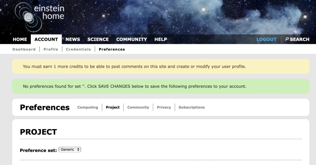
其中,resource share选项代表你愿意与项目分享的算力百分比,默认为百分百,不需要修改,具体的算力占用选项可以在BOINC客户端中设置;
USE CPU选项代表你是否接受基于CPU运行的任务,请根据具体硬件情况选择,如果你使用Apple Silicon芯片,推荐只接受Apple GPU任务;对于大部分平台,勾选CPU和NV GPU是合理的;
在Einstein@home的语境下,具体的计算任务被称为applications:
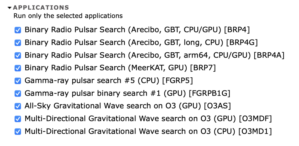
随便选,当然也可以有倾向性地选,最终分配给你的任务是该设置与上一项设置的交集;
接下来是GPU任务的分配,这一项较为重要,它代表你的GPU将并行的任务数,如默认为1,则你的设备将同时运行一个GPU任务;若为0.5,则将同时运行两个。笔者以RTX4000 Ada Mobile (RTX4080 Moble功耗墙换皮卡)测试下,单个任务能吃满算力并占用2GB显存,并行多个任务不会有明显效率提升,不推荐更改该设置;
接下来,我们在BOINC客户端设置客户端的行为,点击option菜单下的computing preference选项,可以选择是否:
在使用主机时停止运行;
在使用主机时停止GPU任务;
在使用电池供电时停止运行;
电脑空闲时最大占用CPU比例和时间;
。。。。
你甚至可以设定BOINC在一天/一周中的哪些时段运行
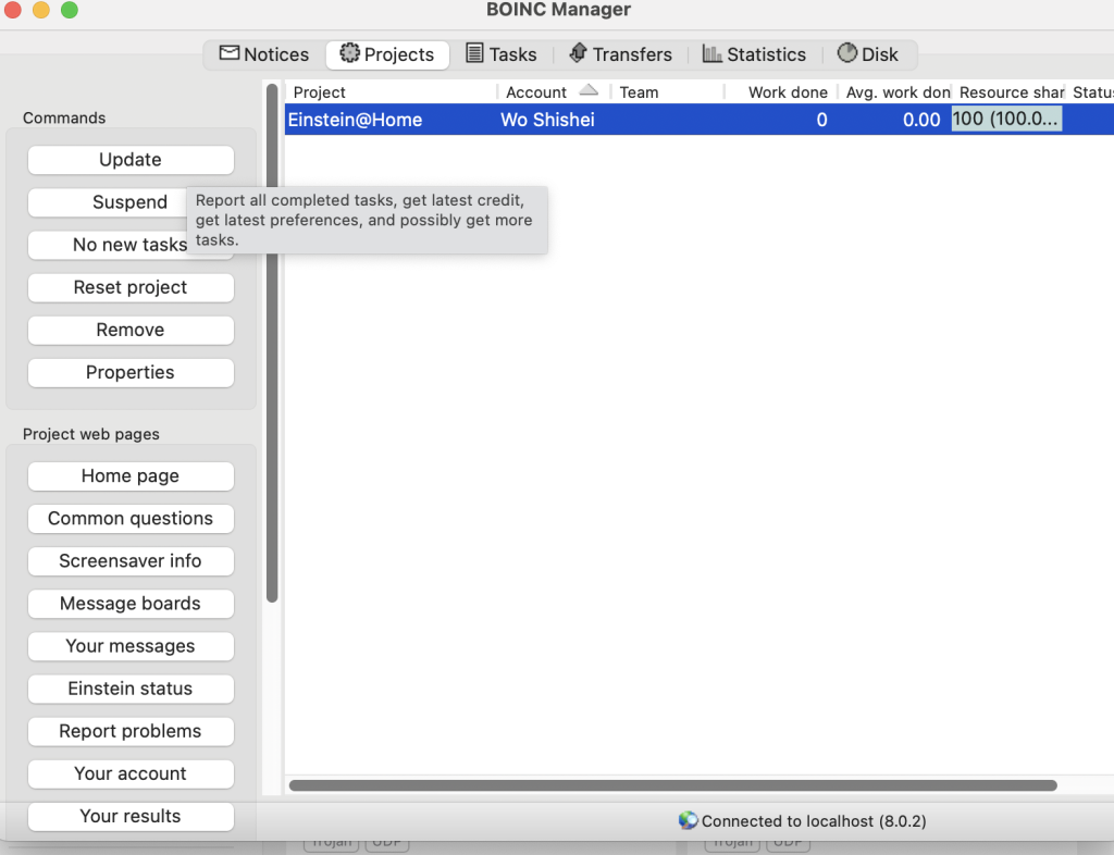
开始工作
选中项目后点击update按钮开始接受任务
加入Physics@WHU
在Einstein@home项目社区https://einsteinathome.org/community/teams可以查找并加入你喜欢的队伍,当然你也可以直接加入Physics@WHU,应该是目前包含Wuhan字段的贡献点最高的队伍吧(应该吧)


